Analytics Engineering with dbt & Databricks: Building a Production-Grade Data Warehouse

Level: Intermediate Data Engineering
Tech Stack: dbt · Databricks · Delta Lake · SQL · Jinja · hive_metastore
Source Code & Practice Files: View on GitHub

The Problem: Raw Data Is Useless

In my beginner pipeline project, we learned how to ingest raw CSV data and clean it with Python. But there’s a critical question that project doesn’t answer:

Once the data is ingested — then what?

In a real company, raw data lands in cloud storage every day. A dozen different analysts and data scientists need to query it — each writing their own transformations, often with subtle differences. One analyst filters out cancelled orders, another doesn’t. One team reports revenue in cents, another in dollars. The result is a classic problem in data teams: everyone has a different number, and nobody knows who is right.

This is the problem that Analytics Engineering — and specifically dbt — was built to solve.

The Solution: A Medallion Architecture on Databricks

Instead of everyone transforming raw data independently, we build a single, shared transformation layer — a structured data warehouse where transformations are:

• Written in SQL (readable by anyone)
• Version-controlled in Git (tracked like application code)
• Automatically tested (data quality is code, not hope)
• Auto-documented (a searchable docs site generated from YAML)

Here is the high-level data flow pipeline, showing the journey from source CSV files all the way to downstream dashboards:

We implement this using the industry-standard Medallion Architecture:

Each layer has a clear contract: Bronze is raw and untouched, Silver is clean and typed, Gold is business-ready and analytical.

The Bronze Layer: Raw Data with Intentional Problems

We load three CSV files into Databricks using dbt seed. Crucially, I’ve designed these files with real-world data quality issues baked in — the same problems you’d encounter in production:

These aren’t mistakes — they’re the teaching material. Every transformation in the Silver layer exists to fix one of these problems.

The Silver Layer: Where the Real Work Happens

The staging models are the heart of this project. Let’s walk through stg_orders.sql in detail:

with source as (
    select * from {{ source('ecommerce_bronze', 'raw_orders') }}
),

-- Step 1: Remove rows with null order_id
filtered as (
    select * from source
    where order_id is not null
),

-- Step 2: Deduplicate — order O001 appears twice, keep the earliest
deduplicated as (
    select * from (
        select *,
            row_number() over (
                partition by order_id
                order by order_date asc
            ) as row_num
        from filtered
    )
    where row_num = 1
),

-- Step 3: Clean and standardize
cleaned as (
    select
        order_id,
        customer_id,
        product_id,
        cast(order_date as date)                    as order_date,
        cast(quantity as int)                       as quantity,
        {{ cents_to_dollars('unit_price_cents') }}  as unit_price,  -- macro!
        upper(trim(status))                         as status,
        lower(trim(payment_method))                 as payment_method
    from deduplicated
),

-- Step 4: Filter negative quantities
final as (
    select * from cleaned
    where quantity > 0
)

select * from final

Notice the pattern: each CTE handles exactly one concern. This is intentional. When a bug appears in production, you trace back through the CTEs one at a time until you find the culprit. Readable SQL is debuggable SQL.

dbt Superpower #1: The Macro

Notice {{ cents_to_dollars('unit_price_cents') }} in the query above. That’s a Jinja macro — a reusable SQL function defined once and used everywhere:

{% macro cents_to_dollars(column_name) %}
    round({{ column_name }} / 100.0, 2)
{% endmacro %}

Why 100.0 and not 100? Because in SQL, dividing an integer by an integer performs integer division — 4999 / 100 = 49 (we lose the cents!). The .0 forces float division: 4999 / 100.0 = 49.99. If you ever need to change the rounding logic, you fix it in one place — not across every model that converts prices.

The Gold Layer: Business-Ready Analytics

fct_orders — The Incremental Fact Table

The fact table joins all three staging models into one enriched, queryable table:

{{ config(materialized='incremental', unique_key='order_id') }}

with orders    as (select * from {{ ref('stg_orders') }}),
     customers as (select * from {{ ref('stg_customers') }}),
     products  as (select * from {{ ref('stg_products') }})

select
    o.order_id, o.order_date, o.quantity,
    o.unit_price, o.quantity * o.unit_price as total_amount,
    o.status, o.payment_method,
    c.full_name as customer_name, c.country as customer_country,
    p.product_name, p.category as product_category, p.brand
from orders o
left join customers c on o.customer_id = c.customer_id
left join products  p on o.product_id  = p.product_id

dbt Superpower #2: Incremental Models

The fct_orders model is materialized as incremental — one of dbt’s most powerful features. Here’s the logic that makes it work:

{% if is_incremental() %}
    where order_date > (select max(order_date) from {{ this }})
{% endif %}

Why does this matter? Imagine your company has 3 years of order history — millions of rows. Without incremental, every dbt run rebuilds the entire table from scratch. That’s expensive, slow, and unnecessary.

With is_incremental():

• First run: Full table build (processes all history)
• Every subsequent run: Only processes orders newer than the latest date already in the table

In production, this cuts a 2-hour full rebuild down to a 3-minute incremental run.

dbt Superpower #3: Testing as Code

This is where dbt changes how you think about data quality. Instead of manually checking tables, you declare your expectations as code in YAML:

- name: stg_orders
  columns:
    - name: order_id
      tests:
        - not_null
        - unique
    - name: status
      tests:
        - accepted_values:
            values: ['DELIVERED', 'SHIPPED', 'CANCELLED', 'RETURNED']

Run dbt test and dbt generates SQL for each test, executes it against your Databricks tables, and reports results:

18 of 18 PASS ............................................................. [PASS in 12.3s]

Done. PASS=18 WARN=0 ERROR=0 SKIP=0 TOTAL=18

We also have a custom singular test for business logic that’s too nuanced for schema tests. The rule: after staging filters, no order should have a negative quantity.

-- tests/assert_no_negative_quantity.sql
-- If this returns ANY rows, the test FAILS.
select order_id, quantity
from {{ ref('stg_orders') }}
where quantity <= 0

These tests run in CI pipelines at real companies. If a test fails, the deployment stops — bad data never reaches analysts.

dbt Superpower #4: The relationships Test (FK Validation)

In the _marts__models.yml, we declare foreign key validation between tables:

- name: customer_id
  tests:
    - relationships:
        to: ref('stg_customers')
        field: customer_id

dbt generates a SQL query that checks: does every customer_id in fct_orders exist in stg_customers? This is the equivalent of a database foreign key constraint — but running as a testable, trackable CI check.

dbt Superpower #4: Source Freshness (dbt source freshness)

Think of this like a freshness sticker on food. You declare a rule: “This data should be updated at least every 24 hours.” dbt then checks the actual timestamp of your source table and tells you whether it is fresh or stale.

In the project, we declare freshness rules on all three Bronze tables:

sources:
  - name: ecommerce_bronze
    freshness:
      warn_after: {count: 24, period: hour}   # yellow warning after 1 day
      error_after: {count: 48, period: hour}  # red error after 2 days
    loaded_at_field: "current_timestamp()"

When you run dbt source freshness, dbt connects to Databricks and checks the timestamp of each source table. You get a clear pass/warn/error result for every one:

✅ PASS  ecommerce_bronze.raw_orders      (updated 2 hours ago)
✅ PASS  ecommerce_bronze.raw_customers   (updated 2 hours ago)
✅ PASS  ecommerce_bronze.raw_products    (updated 2 hours ago)

Why this matters in production: Upstream ETL pipelines fail silently all the time. Without source freshness, your dashboards will show yesterday’s data and nobody will know. A business executive will make a decision based on stale numbers. With dbt source freshness hooked into your monitoring, the data team is alerted before anyone else notices.

dbt Superpower #5: The Auto-Generated Lineage Graph

After running dbt docs generate && dbt docs serve, open localhost:8080 and click the graph icon in the bottom-right. This is what you see:

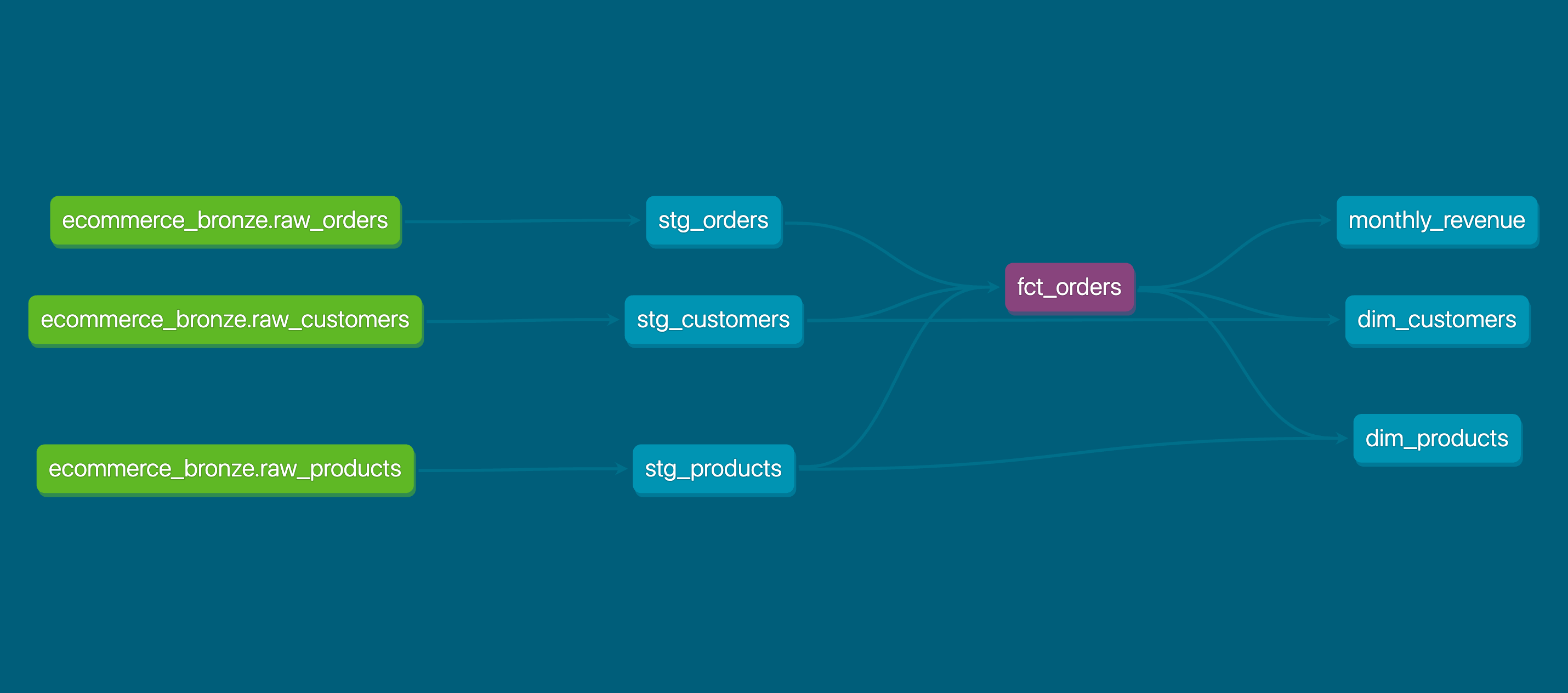
This diagram was generated automatically from your ref() calls in SQL. dbt reads your code, understands the dependencies, and draws this for free. You never have to maintain a data flow diagram again — it updates every time you run dbt docs generate.

Notice fct_orders in the centre (highlighted purple) — it is the hub of the entire warehouse. Three sources flow into it, and three mart tables flow out of it. This is the Medallion Architecture made visible.

The Gold Layer: Dimension Tables

dim_customers aggregates from fct_orders to give each customer a complete business profile:

dim_products similarly aggregates sales metrics per product — total units sold, confirmed units (delivered only), and total revenue.

monthly_revenue is the “executive summary” table: one row per month with order count, unique customers, total revenue, average order value, and the top-performing category for that month — derived using a window function.

SQL Analytics in Databricks

After dbt run, the Gold-layer tables are live and queryable directly in the Databricks SQL Editor. No additional BI tool needed — Databricks has built-in chart visualizations.

Revenue by Payment Method

SELECT
    payment_method,
    COUNT(DISTINCT order_id)    AS total_orders,
    ROUND(SUM(total_amount), 2) AS total_revenue
FROM dev.ecommerce_gold.fct_orders
WHERE status IN ('DELIVERED', 'SHIPPED')
GROUP BY payment_method
ORDER BY total_revenue DESC;

Business insight: Credit card customers account for over 55% of total revenue. A real business would use this to prioritise their payment gateway partnerships.

Product Revenue Performance

SELECT product_name, category, total_revenue, total_units_sold
FROM dev.ecommerce_gold.dim_products
ORDER BY total_revenue DESC;

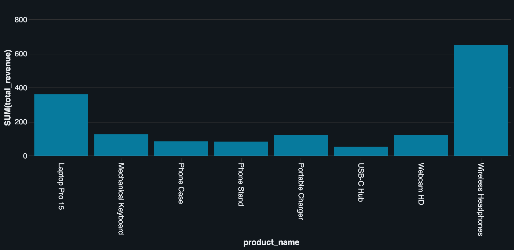
Business insight: Wireless Headphones generates 2x the revenue of the next best product (Laptop Pro 15), despite both being Electronics. This is the kind of signal a product team would act on immediately — expand the headphones range, investigate the laptop.

Customer Lifetime Value

SELECT full_name, country, total_orders, lifetime_value
FROM dev.ecommerce_gold.dim_customers
WHERE total_orders IS NOT NULL
ORDER BY lifetime_value DESC;

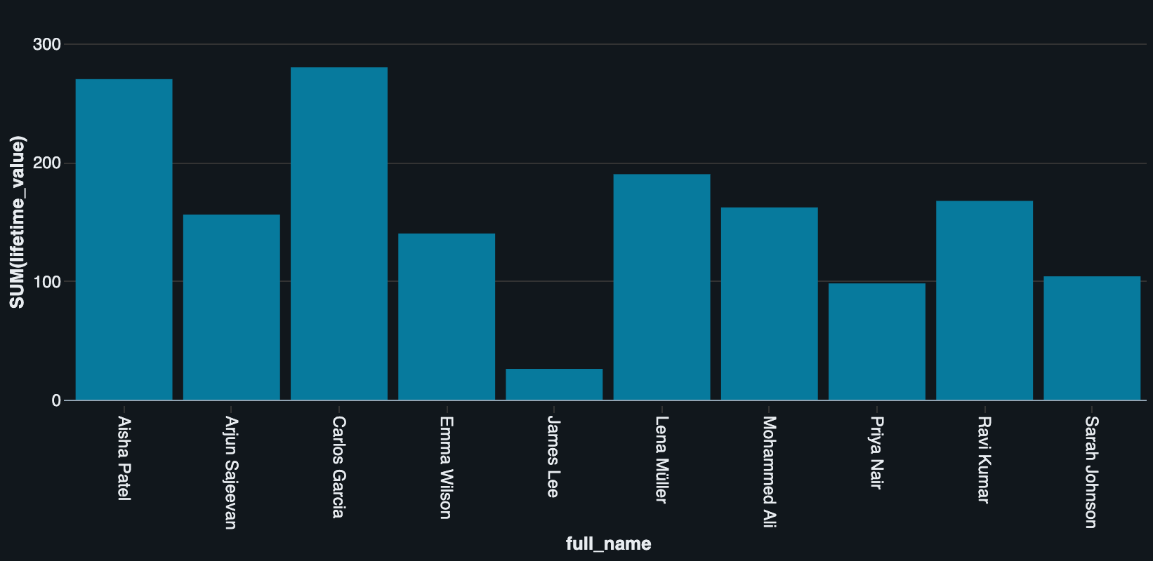
Business insight: The top 3 customers (Carlos Garcia, Aisha Patel, Arjun Sajeevan) each account for over $150 in lifetime value. A retention campaign targeting this cohort would protect a significant portion of revenue.

How to Follow Along

Everything you need is in the GitHub repo. Here’s the full run sequence:

# 1. Install dbt
pip install dbt-databricks

# 2. Copy the profile template and fill in your credentials
cp profiles.yml.example ~/.dbt/profiles.yml

# 3. Install packages
dbt deps

# 4. Test your connection
dbt debug

# 5. Load raw data into Databricks
dbt seed

# 6. Build the warehouse
dbt run

# 7. Run all 18 tests
dbt test

# 8. Generate and explore the docs + lineage graph
dbt docs generate && dbt docs serve

# 9. Check source freshness
dbt source freshness

Then open the Databricks SQL Editor and run the queries in analytics/ to build your charts.

Engineering Decisions

Why views for staging, tables for marts?
Staging models are cheap to recompute — they’re just SQL on top of seeds. Building them as views means they always reflect the latest raw data without using Databricks compute. Marts are queried frequently by dashboards, so they need to be pre-computed tables for fast response times.

Why left join (not inner join) in fct_orders?
An inner join would silently drop orders if a customer_id or product_id doesn’t match — a data loss bug that’s hard to detect. Left join preserves all orders and leaves customer/product columns null if there’s no match. The relationships test then catches these orphaned records explicitly.

Why is the monthly_revenue model not incremental?
Monthly aggregates need to be recalculated whenever historical data changes (late-arriving orders, status updates). An incremental strategy would be wrong here — we need a full rebuild to get accurate monthly totals. For a 3-month dataset, a full rebuild takes milliseconds anyway.

Key Takeaways

1. dbt makes SQL a first-class engineering artifact. Version-controlled, tested, documented SQL is fundamentally different from ad-hoc queries.

2. The Medallion Architecture is not just a pattern — it’s a contract. Every layer has a specific responsibility. Bronze is raw, Silver is clean, Gold is business-ready.

3. Incremental models are the difference between a pipeline and a production pipeline. Always ask: “Do I need to reprocess historical data on every run?”

4. Test your data like you test your code. dbt test in CI means data quality failures block deployments — exactly like unit test failures.

5. Documentation is a deliverable, not an afterthought. The dbt docs site is the gift you give to every analyst who comes after you.

Project Resources

Ready to build this yourself? Everything is in the repo — seeds, models, macros, tests, and analytics SQL files.

👉 View the Full Project on GitHub